This is a quick look at the technique I used when competing in the Kaggle Galaxy Zoo competition a while back (https://www.kaggle.com/c/galaxy-zoo-the-galaxy-challenge). I thought it would be a helpful, basic look into using scikit image for image segmentation. The image segmentation technique here is performed by identifying a region of interest (ROI) and creating a mask that will be used to isolate that region from the remainder of the image.
from skimage import io, color
import matplotlib.pyplot as plt
%matplotlib inline
import skimage.morphology as morph
from skimage.measure import label
from skimage.filters import threshold_otsu
import numpy as np

def plot_image(data, title):
""" This function is used to plot the images used in this example.
:param data: image file
:param title: string to use as the plot title
"""
plt.figure(figsize=(7,7))
io.imshow(data)
plt.axis('off')
plt.title(title)
plt.show()
First we need to load the original image.
fileName = '104682.jpg'
picOriginal = io.imread(fileName)
plot_image(picOriginal, 'Original')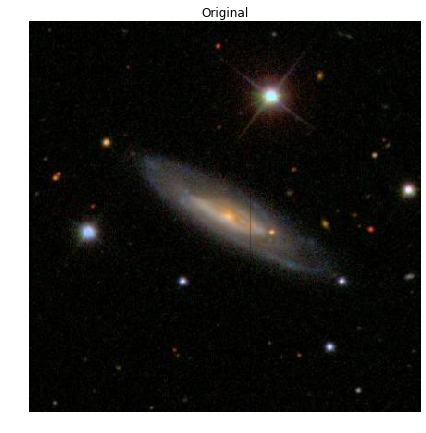
The first step into building the segmentation mask is to convert the RGB image to a grayscale image.
picGray = color.rgb2gray(picOriginal)
plot_image(picGray, 'Grayscale')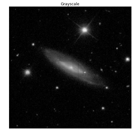
Next, we need to convert the grayscale image to a binary image so we can perform some morphology on the image. While it is possible to perform morphology on grayscale images, binary images are simpler to deal with and easier to understand what’s going on.
To convert the image, we use the Otsu’s Threshold method (https://en.wikipedia.org/wiki/Otsu%27s_method). This method is used because it’s a parametric method to select a threshold value that basically maximizes the variance between the light and dark pixels in the resulting image.
Thresh = threshold_otsu(picGray)
picBW = picGray > Thresh
plot_image(picBW, "B&W")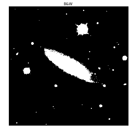
The regions in the resulting binary image are called blobs. The trick here is to 1) isolate the blob we care about and 2) make sure that blob isn’t connected to any other blobs we don’t. To do this, we have to perform some morphology on the image; that is erosion, dilation, closing and opening which are applied to the image using structuring elements. (https://en.wikipedia.org/wiki/Mathematical_morphology)
This part is the where magic happens, since the morphology performed on one image may not be right for another. Depending on the application, measures against this can be put in place.
The structuring elements used here are disks of two sizes. One with a 2-pixel radius and one with a 5-pixel radius.
Strel = morph.disk(2)
Strel2 = morph.disk(5)
plt.figure(figsize=(7,7))
plt.subplot(131)
plt.imshow(Strel)
plt.title("2-Pixel Radius Disk Element")
plt.subplot(133)
plt.imshow(Strel2)
plt.title("5-Pixel Radius Disk Element")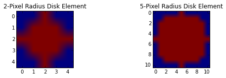
A dilation is performed using the 2-pixel disk element. This is to elarge the blobs in order to capture all of the small specs around the galaxy. You can see also see an increase in the size of all of the individual blobs.
BWimg_dil = morph.dilation(picBW,Strel)
plot_image(BWimg_dil, "Dilated")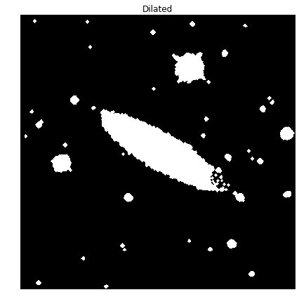
The last thing we have to capture, of the ROI, is the region on the right that seems a bit too open. To capture this area in our blob, we need to close this area. We do this using the 5-pixel radius disk element and the closing morphological function.
BWimg_close = morph.closing(BWimg_dil,Strel2)
plot_image(BWimg_close, "Closed")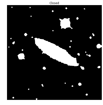
Now that we have the area we want isolated, it’s time to segment that region from the rest. We do this by applying a lable to each of the blobs and selecting the one we want. In this case, we want the blob that intersects with the center of the image (an assumption for this competition was that the galaxy of interest was in the center of each image).
L = label(BWimg_close)
plot_image(color.label2rgb(L), 'Labeled Regions')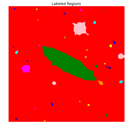
half_length = int(np.floor(np.size(L,1)/2))
L_cntr = L[half_length,half_length]
print "Label of blob that contains the center pixel: {}".format(L_cntr)
Label of blob that contains the center pixel: 14
Once we know the label of the blob that contains the center pixel, we want to set all pixels with that label to 1 and the rest equal to 0 to create a mask of the ROI.
Seg = L
Seg[Seg != L_cntr] = 0
Seg[Seg == L_cntr] = 1
plot_image(Seg, 'ROI')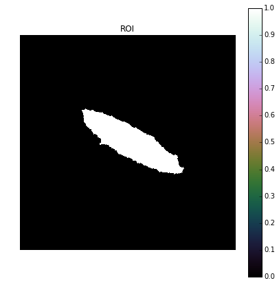
Now that we have our mask, we can make it slightly more robust by increasing the size of the ROI so that it covers a little extra area. To do that we perform another dilation using the 5-pixel radius disk element.
Mask = morph.dilation(Seg,Strel2)
plot_image(Mask, "Mask")
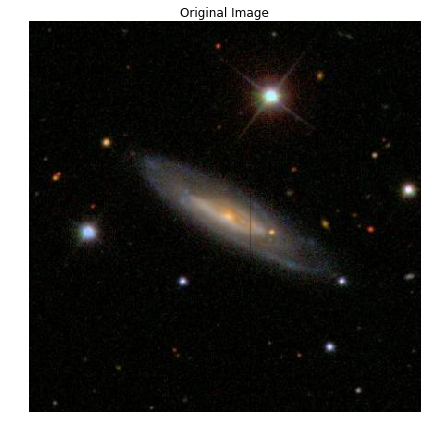
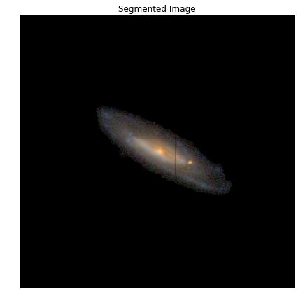
Now that we have our final mask, all we have to do is apply it to the original image. This is done by finding all of the coordinates for the pixels outside of the ROI and then we remove those same pixels from the original image by setting them equal to 0.
[indx, indy] = np.where(Mask == 0)
Color_Masked = picOriginal.copy()
Color_Masked[indx,indy] = 0
plot_image(picOriginal, "Original Image")
plot_image(Color_Masked, "Segmented Image")